Litnet

Abstract

Suggested citation: The citation should list the original Afrikaans paper, followed by the link to this abstract in English.
Note: This tightly constrained English abstract is in point form. Software and additional information with which to replicate the examples can be found here.

1. Introduction

Extended exploration of financial time series, using my own software, provided evidence of structure in prices of financial markets. Prices tend to change direction repeatedly along specific straight lines to indicate the presence of preferred gradients (Joubert 1993, 1994).

1.1 Three instances of a preferred gradient located in prominent points on a price chart form a channel pair. The channel ratios identified in all financial time series are 500:500, 382:618, 400:600, 300:700, 200:800, 150:850, 100:900, 333:667 and 236:764. 

1.2 Different preferred gradients are related through the Fibonacci ratio. Changing a known gradient by this ratio delivers another preferred gradient. Repeated transformations deliver a “family” of gradients that differ by at least 61,8%.

An algorithm based on these two features is used to create bias-neutral examples which demonstrate the existence of a consistent and accurate phenomenon.

2. The analysis of preferred gradients

Prices change direction at preferred gradients. In Diagram 2.1, V1 is a known preferred gradient with V2 unknown. Diagram 2.1A, a “goodbye kiss” on V1, occurs in a sustained trend. Diagram 2.1B is a bifurcated low, with its inverse being a bifurcated top. The centre reversal of bifurcated patterns typically identifies important preferred gradients.

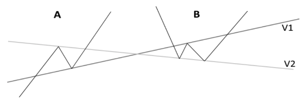
Diagram 2.1. Standard interactions between price and preferred gradients

The algorithm used to create the examples consists of two steps: 

2.1 Define a master gradient between two prominent points on the chart: The gradients of all other trend lines are derived from this to enforce only one family of gradients being used in an example.

2.2 Search systematically for three instances of a derived gradient located in prominent chart points that have a known ratio. 

Once a master gradient is defined, the ratios of all such derived channel pairs to be found by a mechanistic search are predetermined. Only three commonly seen ratios – 500:500, 382:618 and 400:600 – qualify to determine whether the algorithm correctly represents features of the phenomenon. Acceptable channel ratios may not differ by more than 9 places in the third decimal from a known ratio (±1%).

3. Examples

An x identifies anchor points used for the master gradient; an o identifies the locations of derived trend lines. When the initial trend lines of channel sets are located in the first data point, these may not be visible. Examples employ the monthly averages of the S&P500 index, price of gold in euro, Swiss franc-US dollar and US dollar-SA rand exchange rates, and the daily Dow Jones Industrial Average (FRED, Quandl).

3.1 Master gradient defined between prominent lows on the chart

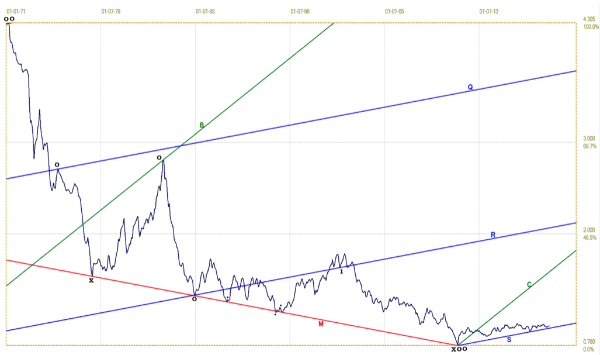
Example 3.1. Swiss franc-US dollar exchange rate. January 1871 to November 2019

ABC 384:616, PQR 506:494 and QRS 602:398

Line R differs by 0,05% from the central point of bifurcated top 1, expressed in terms of the vertical scale. The difference must be less than 0,5% to qualify as an intersection.

Even quite minimal changes to any of the sets of coordinates of time and price of the six anchor points will collapse the specific relationship between the sets of coordinates that makes this example possible.

Example 3.2 Master gradient defined between the 1929 and 1987 highs

Example 3.2. S&P500 (1). January 1871 to June 2019

ABC 500:500, BCD 500:500, PQR 398:602 and XYM 380:620

Channel set ABCD is symmetrical, which confirms the location of line C.

Example 3.3 Master gradient defined between first data point and September 2012 high

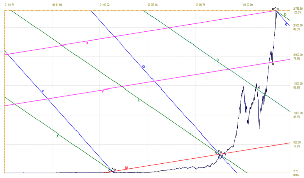
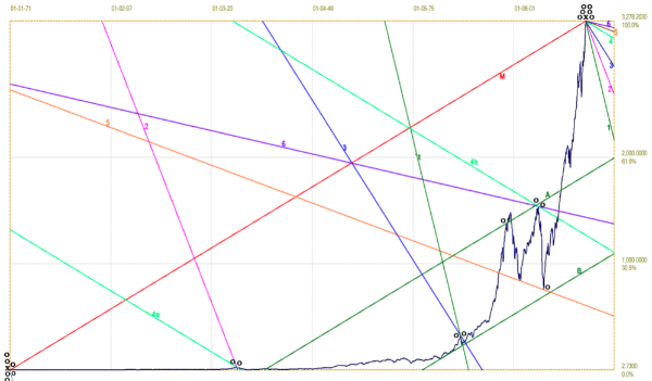
Example 3.3. Gold price in D-mark/euro. January 1971 to April 2020

ABC 499:501. PQR 395:605 and XYZ 379:621

The D-mark and euro time series were normalised before calculating the gold price.

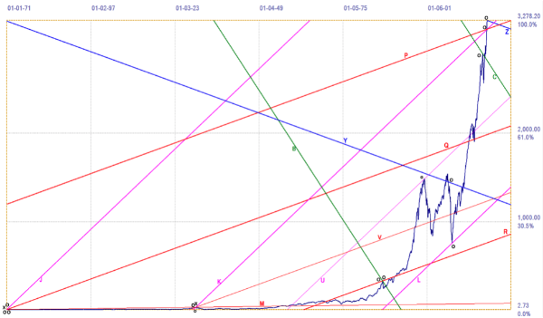
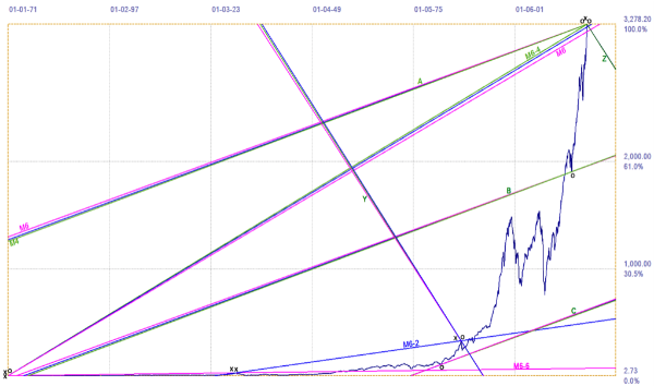
Example 3.4 Master gradient defined between January 1871 and January 2020

Six channel pairs and one channel set of 4 trend lines are located between the first data point and the January 2020 high.

Example 3.4. S&P500 (2). January 1871 to January 2020

MAB 617:383, 111 594:406, 222 320:680, 333 406:594, 444a 290:710, 444b 616:384, 555 496:504 and 666 593:407

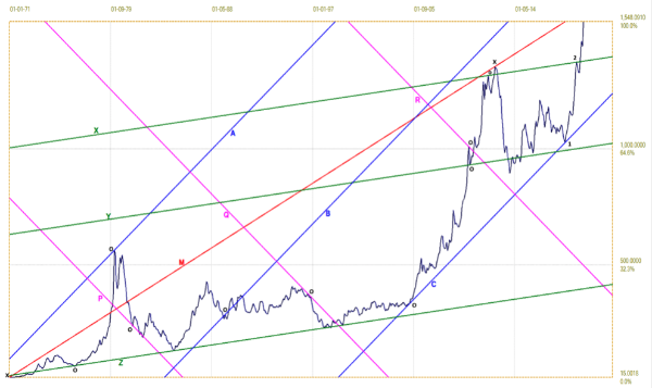
Example 3.5 Master gradient defined between first data point and January 2016 high

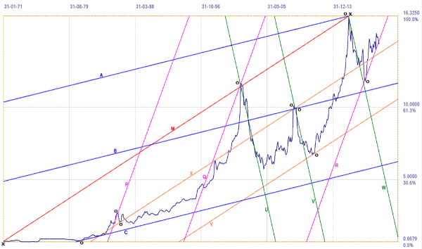
Example 3.5. US Dollar-SA Rand exchange rate. January 1971 to January 2020

ABC 502:498, MXY 496:504, PQR 382:618 and UVW 399:601

Lines X and B are located in bifurcated tops.

Example 3.6 Master gradient defined between first data point and 1929 high

Channels KL and QR of the four main channel pairs are divided by additional trend lines U and V. Trend lines K and B are 76 and 123 times steeper than the master gradient. 

Example 3.6. S&P500 (3). January 1871 to January 2020

Primary channel pairs: ABC 615:385, JKL 503:497, PGR 507:493 and XYZ 622:378
Secondary channel pairs: JKU 665:335, KUL 497:503, PQV 613:387 and QVR 615:385

All eight ratios are known, but JKU with a 1/3:2/3 ratio does not qualify.

Example 3.7 Master gradient defined between the first data point and March 2009 low

The DJIA time series spans 120 years (33 568 days) since 14 July 1896. Some trend lines of the four main channel sets are not visible. Channel pairs XWY and YVZ are two additional channel pairs. Line Q is located in the central point of a bifurcated low in March 2009.

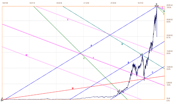
Example 3.7. Dow Jones index. Daily closing values from 14 July 1896 to 19 March 2020

ABC 614:386, JKL 504:496, PQR 695:305, XYZ 497:503, XWY 700:300 and YVZ 401:599

Channel pairs XWY and YVZ confirm that line Y is correctly located. The gradients of pairs XYZ and JKL differ by two Fibonacci transformations, which require different locations for lines K and Y for both ratios to correspond to 500:500.

4. The sensitivity of preferred gradients for changes in gradient

It happened inadvertently that the master gradients in Examples 3.2, 3.4 and 3.6 belong to the same or similar families of gradients, as illustrated in Example 4.1.

Example 4.1 Three master gradients of Examples 3.2, 3.4 and 3.6

Steeper derivatives of master gradients M3-2 and M3-6 are similar to the master gradient M3-4 of Example 3.4. 

Example 4.1. Comparison of three S&P500 master gradients

Table 4.1 shows the ratios of channel pairs ABC and XYZ of the different master gradients are closely similar. 

Table 4.1. Channel ratios of three different master gradients

Steeper derived lines of M3-2 and M3-6 miss the January 2020 high (where M3-4 is defined by 0,79% and 2,74% respectively). This is too far for an interception.

Example 4.1 demonstrates that channel ratios cannot distinguish between closely similar families of gradients, while the fit of derived trend lines to the chart can do so. However, using trend lines has limitations of scale. Example 4.1 suggests the phenomenon has a fine structure.

Example 4.2 S&P500 (4). A fourth master gradient between January 1871 and October 2007

This proves that the results of other S&P500 examples do not rely on the similarity of their master gradients. It also employs the January 2018 high instead of the September 2018 high.

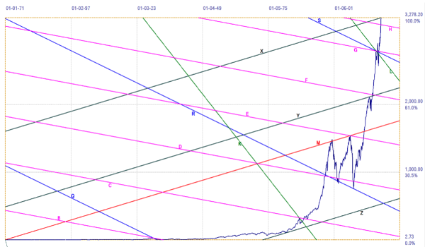
Example 4.2. S&P500 (4). January 1871 to January 2020

JKL 600:400, XYM 696:304, YMZ 298:704, PQR 335:665 en QRS 497:503, ABC 383:617, BCD 505:495, CDE 508:492, DEF 501:499, EFG 496:504 and FGH 621:317

All 11 channel ratios are known, but three do not qualify. The ratios of pairs XYM and YMZ are both similar and reversed to make channel set XYMZ symmetrical. Pair PQR has the known 1/3:2/3 ratio. Five ratios correspond to 500:500, two to the Fibonacci ratio; one is 400:600. The set ABCDEFGH is symmetrical to confirm that trend lines F and H are correctly located.

With some lines removed, the remaining sets ACDEFH and ABDEGH also display known ratios.

ACD 623:377, EFH 387:613, ABD 238:762, EGH 768:232.

Both symmetrical sets consist of two channel pairs separated by channel DE. Pairs ABD and EGH do not qualify for the test. Their ratios correspond to the 236:764 ratio of the third power of the Fibonacci ratio (0.618034).

Example 4.2 illustrates that the good ratios from the other S&P500 examples do not result from the close relationship between their master gradients.

5. Discussion of the examples 

The examples were designed to substantiate the claim that preferred gradients are a feature of different time series. The algorithm used for the examples ensures compliance with what is known of the phenomenon and is bias neutral, except for the definition of the master gradient. 

Table 5.1. Distribution of channel ratios in the examples

Table 5.1 shows the distribution of the ratios in the examples (S&P500 examples in red). Eight of 54 channel pairs do not qualify, so that 46 (85%) of the ratios satisfy the test requirements. The presence of the phenomenon of preferred gradients as defined by its features encoded in the algorithm is confirmed in all five time series. 

Table 5.2. Distribution in the S&P500 examples of 10 prominent anchor points

The first column of Table 5.2 shows the dates and usage count of ten prominent chart points used to locate 61 of the 69 anchor points in the examples based on the S&P500 time series. This supports evidence in Table 5.1 that the algorithm correctly interprets the observed features of the phenomenon. 

In Example 3.7, the master gradient uses the low on 9 March 2009. Its coordinates of time and price are not the result of normal market forces, but of the decision by the US Federal Reserve to intervene in the financial crisis by injecting funds into financial markets (Yahoo Finance 2009). The S&P500 examples therefore imply that this phenomenon accommodates trend reversals whether due to normal market forces or intervention.

6. Conclusions 

Table 5.1 shows that the algorithm was successful in terms of its objective to confirm that the two features of the phenomenon used for the algorithm reflect the presence of structure in all five time series. 

The hypothesis that all trend changes occur at preferred gradients implies that the random changes of market prices result from a similar mechanism as the Brownian movement of a molecule in a gas (Encyclopaedia Britannica 2018).

The observed structure in the examples is assumed to be evidence of emergence in financial markets as complex self-adaptive systems, as described here:

When electrons or atoms or individuals or societies interact with one another or their environment, the collective behaviour of the whole is different from that of its parts. We call this resulting behavior emergent. Emergence thus refers to collective phenomena or behaviors in complex adaptive systems that are not present in their individual parts. (Pines 2014)

Keywords: chart patterns; complexity; Dow Jones Index; Efficient Market Hypothesis; euro; Fibonacci ratio; financial markets; gold price; monthly averages; preferred gradients; S&P500 Index; South African rand; structure in market prices; Swiss franc; time series

Lees die volledige artikel in Afrikaans

Waarnemings van langdurige struktuur in tydreekse van finansiële markte